Frequentist inference

Frequentists answer questions about populations using data from samples. In the frequentist framework, population parameters are treated as fixed but unknown quantities. They take a random sample from the population to make inferences about the population.

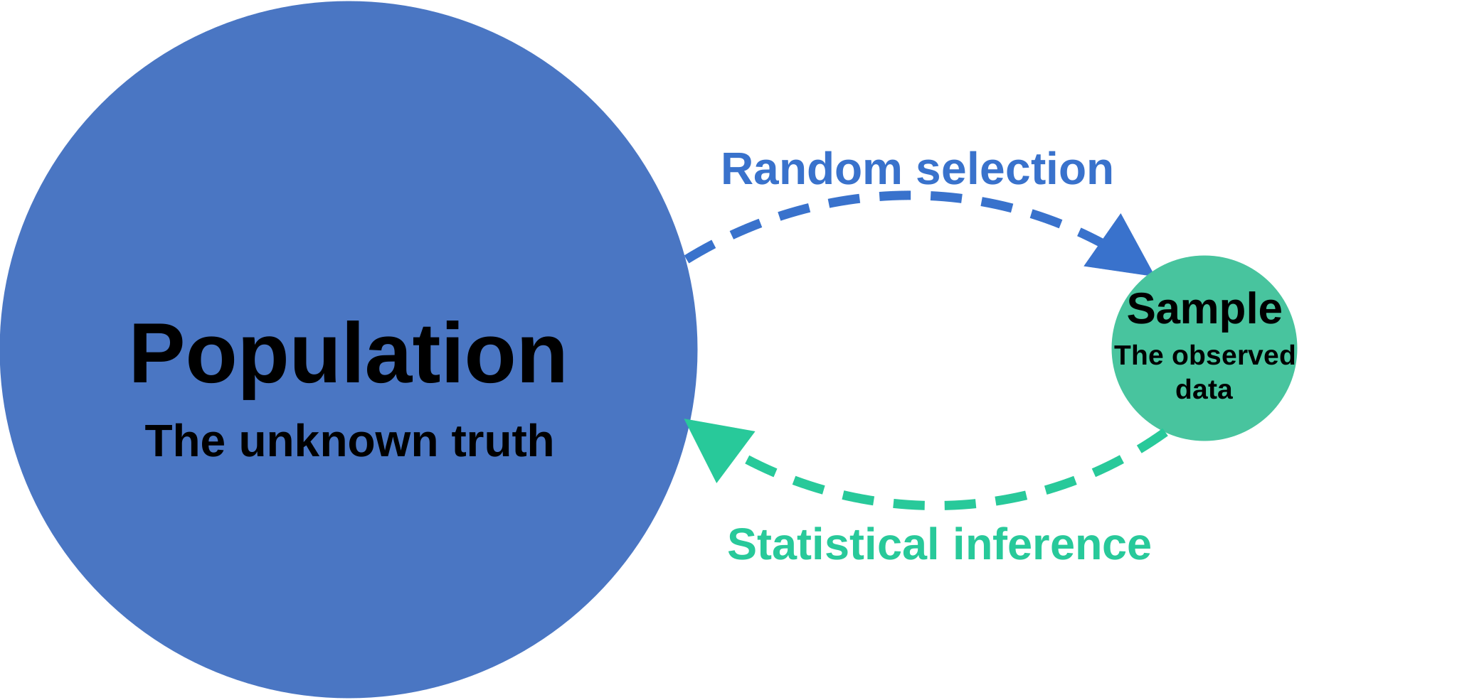
The key to frequentist inference is the sampling distribution. We use sampling distributions to estimate standard errors, construct confidence intervals, and calculate p-values. The sampling distribution is the distribution of a statistic (like the mean) over repeated samples from the same population.

To demonstrate the sampling distribution, we can use a simulation. In this simulation, we will take 1000 samples of size 10 from a population. We will calculate the mean of each sample and plot the distribution of the sample means.

First, we start by simulating a population. In this case, we will simulate a population of 1 million people with heights that are normally distributed with a mean of 70 inches and a standard deviation of 3 inches. We'll name the current frame 'population'.

. clear

. set seed 89320

. set obs 1000000
Number of observations (_N) was 0, now 1,000,000.

. generate x = rnormal(70,3)

. frame rename default population

Next, we'll create a new frame called 'sample' and put a sample of size 10 from the population into the sample frame.

. preserve

. sample 10, count
(999,990 observations deleted)

. frame put *, into(sample)

. restore

We can calculate the mean of the sample and use it to estimate the mean of the population.

. frame sample: summarize x

    Variable |        Obs        Mean    Std. dev.       Min        Max
-------------+---------------------------------------------------------
           x |         10    70.86198    1.991961   67.79588    72.9367

In this case, the sample mean is 70.9 inches. In real life, this sample is the only information we would have about the population, and so we would use the sample mean to estimate the population mean. But how accurate is this estimate? To answer that question, we need a sampling distribution.

A sampling distribution is the distribution of a statistic (like the mean) over repeated samples from the same population. To approximate the sampling distribution, we will take 1,000 samples of size 10 from the population and put the sample means into a new frame called 'sampling_distribution'.

. frame create sampling_distribution mean

. forvalues i = 1/1000 {
  2.   preserve
  3.   quietly sample 10, count
  4.   quietly summarize x
  5.   frame post sampling_distribution (r(mean))
  6.   restore
  7. }

To see the sampling distribution of the sample means, we create a histogram.

. frame sampling_distribution: histogram mean
(bin=29, start=67.261787, width=.20027739)

This histogram approximates the sampling distribution of the mean using 1,000 samples of size 10. It shows how sample means vary around the population mean. We quantify this variability with the standard error of the mean, which is the standard deviation of the sampling distribution.

. frame sampling_distribution: summarize mean

    Variable |        Obs        Mean    Std. dev.       Min        Max
-------------+---------------------------------------------------------
        mean |      1,000    69.97678    .9429096   67.26179   73.06983

The standard deviation of these 1,000 sample means is 0.94 inches, which approximates the standard error of the mean. Across repeated samples of size 10, the sample means have a typical spread of about 0.94 inches around the population mean.

Again, in real life, we would not have access to the sampling distribution. However, we can estimate its standard deviation—the standard error of the mean—from our sample. For a simple random sample from a population much larger than the sample, we estimate the standard error by dividing the sample standard deviation by the square root of the sample size.

. frame sample: summarize x

    Variable |        Obs        Mean    Std. dev.       Min        Max
-------------+---------------------------------------------------------
           x |         10    70.86198    1.991961   67.79588    72.9367

. display r(sd)/sqrt(r(N)) 
.62991328

For this particular sample, the estimated standard error is 0.63 inches. This differs from the approximate standard error obtained in our simulation. An estimated standard error will itself vary from sample to sample. There are many other types of samples and corresponding formulas for standard errors, but this is one of the simplest.

In conclusion, frequentist inference allows us to make statements about population parameters based on sample data, by using the standard error to quantify the uncertainty in our estimates.