Bayesian inference

Bayesian inference uses data to update what we know about an unknown quantity. It combines a prior distribution with a model for the observed data—the likelihood—to produce a posterior distribution.

$$ p(\boldsymbol{\theta} \mid \mathbf{X}) = \frac{p(\mathbf{X} \mid \boldsymbol{\theta})p(\boldsymbol{\theta})} {p(\mathbf{X})} $$

This is the mathematical representation of Bayes' theorem in the context of Bayesian inference. Let's break down what each of the components represents:

p(θ | X) is the posterior distribution: what the model says about the unknown parameter θ after seeing the data X.
p(X | θ) is the likelihood: how compatible each possible value of θ is with the observed data.
p(θ) is the prior distribution: what the model says about θ before seeing the current data.
p(X) is the marginal probability of the data. It scales the numerator so the posterior is a proper probability distribution.

The marginal distribution of the data, p(X), serves as a normalizing constant to ensure that the posterior distribution sums to one over all possible parameter values. As such, Bayes' theorem is often written in a proportional form as:

$$ p(\boldsymbol{\theta} \mid \mathbf{X}) \mathrel{\Large\propto} p(\mathbf{X} \mid \boldsymbol{\theta})p(\boldsymbol{\theta}) $$

In words: posterior ∝ likelihood × prior. The posterior is our updated description of the parameter, including both a central estimate and the uncertainty around it.

Let's do a simple example.

Suppose we have a coin and we want to estimate the probability of it landing heads.

Let θ be the coin's probability of landing heads. We will start with a Beta(1, 1) distribution. This is a uniform prior: every value of θ from 0 to 1 has equal density. Its mean is 0.5, but it does not favor 0.5 over other possible values.

$$ p(\theta) = \text{Beta}(1, 1) $$

Now I flip the coin 10 times and observe 7 heads and 3 tails. The sample proportion is 7/10 = 0.70. I put the data into Stata, using 1 for heads and 0 for tails.

. clear

. input heads

         heads
  1. 1
  2. 1
  3. 0
  4. 1
  5. 1
  6. 1
  7. 0
  8. 0
  9. 1
 10. 1
 11. end

Because each outcome is 0 or 1, I model each flip with a Bernoulli likelihood with probability θ.

I combine my prior belief with the observed data using the bayesmh command in Stata.

. bayesmh heads, likelihood(dbernoulli({p})) prior({p}, beta(1,1)) rseed(1234)

Burn-in ...
Simulation ...

Model summary
------------------------------------------------------------------------------
Likelihood: 
  heads ~ bernoulli({p})

Prior: 
  {p} ~ beta(1,1)
------------------------------------------------------------------------------

Bayesian Bernoulli model                         MCMC iterations  =     12,500
Random-walk Metropolis–Hastings sampling         Burn-in          =      2,500
                                                 MCMC sample size =     10,000
                                                 Number of obs    =         10
                                                 Acceptance rate  =      .4419
Log marginal-likelihood = -7.2012826             Efficiency       =      .2233

------------------------------------------------------------------------------
             |                                                Equal-tailed
             |      Mean   Std. dev.     MCSE     Median  [95% cred. interval]
-------------+----------------------------------------------------------------
           p |  .6689006   .1337774   .002831   .6781534   .3855673   .9000232
------------------------------------------------------------------------------

The model summary confirms the Bernoulli likelihood and Beta(1, 1) prior. The next lines describe the Markov chain Monte Carlo (MCMC) calculation that Stata used to approximate the posterior.

For this example, we can also derive the posterior exactly. A Beta prior combined with Bernoulli data produces another Beta distribution. We add the 7 heads to the first prior parameter and the 3 tails to the second:

$$ \theta \mid X \sim \operatorname{Beta}(1+7,\,1+3) = \operatorname{Beta}(8,4) $$

The posterior mean is 8/(8+4) = 0.67, which agrees with Stata's simulation-based estimate. This does not mean that the posterior probability of heads is a single number. The posterior is the entire Beta(8, 4) distribution; 0.67 is one useful summary of it.

The sample proportion is 0.70. The posterior mean is slightly closer to 0.50 because the prior contributes a small amount of information. With more flips, the data would have more influence and the prior would matter less.

We can visualize this posterior distribution to better understand our uncertainty about the probability of heads using the bayesgraph command in Stata.

. bayesgraph histogram {p}

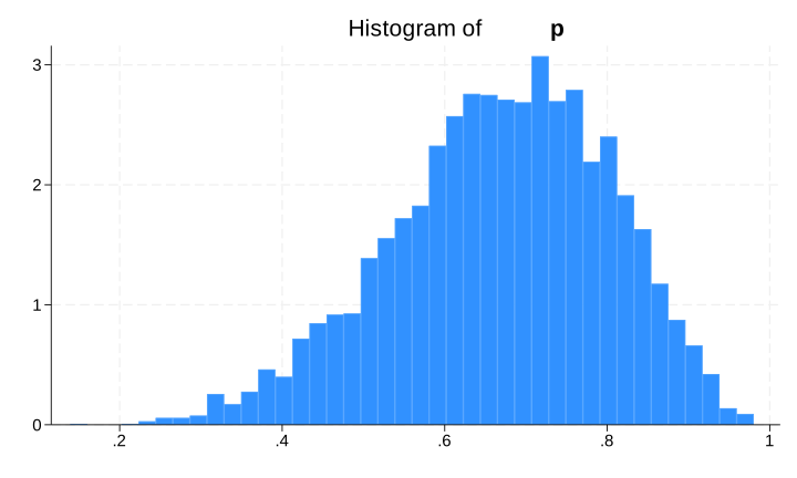
This is a histogram of the posterior distribution. It represents our uncertainty about the probability of the coin landing heads.

We can use the mean, median, or mode as a point estimate for the probability of heads.
The posterior standard deviation describes the remaining uncertainty about θ.
We can use the 2.5th and 97.5th percentiles to form a 95% credible interval for the probability of heads.

We can also ask a direct probability question: given our model and data, what is the posterior probability that θ is greater than 0.50? The bayestest interval command estimates it.

. bayestest interval {p}, lower(.5)

Interval tests     MCMC sample size =    10,000

       prob1 : {p} > .5

-----------------------------------------------
             |      Mean    Std. dev.      MCSE
-------------+---------------------------------
       prob1 |     .8867     0.31698   .0064305
-----------------------------------------------

Under this model, the posterior probability that θ is greater than 0.50 is about 0.89. This statement is conditional on the prior, likelihood, and observed data.

In conclusion, Bayesian inference combines a prior and a likelihood to produce a posterior distribution. That distribution lets us summarize a parameter, describe our uncertainty, and answer probability questions about the parameter directly.